Monte Carlo
While approximation methods exist for some option types using partial differential equations. However, given a model for the option’s underlying asset a Monte Carlo simulation can be created quite easily. Such is the case for options on equities for which Geometric Brownian Motion is often used (or some variation on that model). Given a probability distribution for price changes, a sample price path can easily be created. The payoff function for the option type can then be used to determine the price for the option. If this is repeated enough times, the average of the calculated option prices will asymptotically converge to the true price. Below we compare the accuracy of the Monte Carlo method relative to the closed-form Black-Scholes equation if we keep all of the parameters constant.
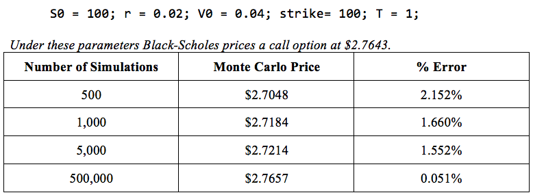
As seen, a higher number of simulations will produce a value closer to the expected value. However, even with 500,000 simulations there still exists a significant amount of error. Monte Carlo simulations may not always be the most accurate unless a large number of sample paths are simulated, but for some option types there is not always an alternative. For retail investors who do not always worry about a $0.01 price difference in financial products, Monte Carlo simulations can be very helpful in pricing options.
Implied Volatility Comparison
Using the historical data described earlier, we calibrated our Black-Scholes model’s volatility parameter. Below, the implied volatility and our calibrated volatility for two separate dates are shown below.
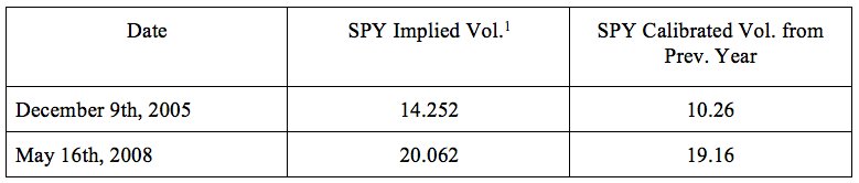
1 Bloomberg
From the data above, we can hypothesize that the implied volatility of the option is not directly linked to the historical volatility of the past year. This means that market participants do not think that the behavior of the underlying asset over the previous year will predict its behavior in the future.
Price Bands
Although Geometric Brownian Motion is used to model stock prices in the Black-Scholes model, there are some pitfalls that make the Geometric Brownian Motion model not the most realistic model of stock price behavior. First, the Geometric Brownian Motion model assumes that the volatility of the underlying stock price (σ) remains constant over time, however as we know from observing real stock prices this is not case. Secondly, GBM processes follow a continuous path and thus does not account for major changes in stock prices caused by unpredictable news or events.
In order to show this we used the implied volatility and found that the actual movement of the stock price does not necessarily follow the expected price movement at the beginning of the contract. We constructed graphs of the underlying stock price over the life the of the option with bands representing the three standard deviation ranges of the stock price keeping the implied volatility of the option constant. We also used the prior year’s historical data in order to calculate the percentage drift of the stock price which also we held constant. For the normal trading year with the contract starting on 12/09/2005 we observed the following:
In order to show this we used the implied volatility and found that the actual movement of the stock price does not necessarily follow the expected price movement at the beginning of the contract. We constructed graphs of the underlying stock price over the life the of the option with bands representing the three standard deviation ranges of the stock price keeping the implied volatility of the option constant. We also used the prior year’s historical data in order to calculate the percentage drift of the stock price which also we held constant. For the normal trading year with the contract starting on 12/09/2005 we observed the following:
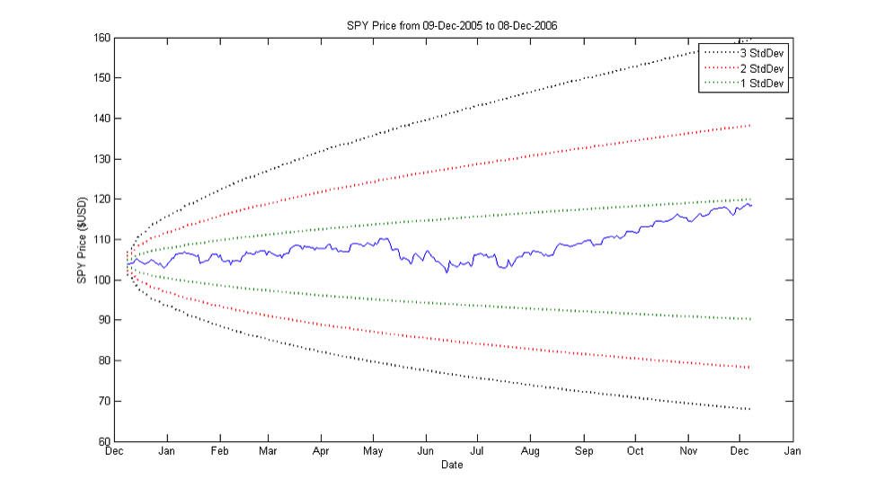
As you can see from the graph, the price of SPY stays within the one standard deviation price band throughout the life of the contract. This makes sense because there was no real unexpected market crashes or news throughout the life of the contract and thus the Black-Scholes model holds. These are ideal conditions for the Black-Scholes model because of low volatility and no major market crashes.
We then observed the movement of the stock price during the financial crisis with a contract written on 05/16/2008:
We then observed the movement of the stock price during the financial crisis with a contract written on 05/16/2008:
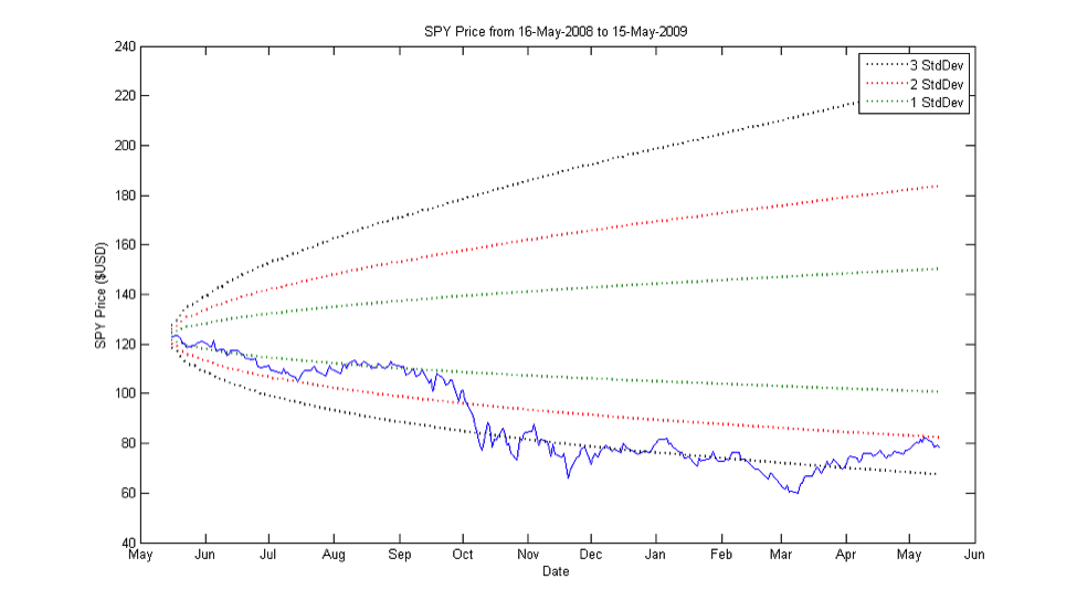
Prior to mid-September 2008, the stock price seems to be stable and the Black-Scholes model is seeming hold. However as the financial crisis starts to hit and investors panic there is an extreme increase in the underlying stock’s volatility which send the stock price plummeting. The stock price of SPY hits about 4.25 standard deviations from the expected price at its minimum, which means that this should happen roughly once in every 16,500 years. As we know from history, financial crashes like these actually occur at a much higher frequency. Between the Wall Street Crash of 1929 and the Great Depression, Black Monday in 1987, the Savings and loans crisis, and the Dot-com bubble the US financial markets have seen their fair share of events like these only within the past 100 years. This shows that the probability distribution of price under the Black-Scholes model does not always represent the actual movement of prices in the market, especially when looking at major price movements.
Model Comparison
While calibrating the Heston model was outside the scope of this project, we were able to qualitatively compare the Heston model to the Black-Scholes model by analyzing their response to changes in a single parameter as the others remained constant. First, we looked at how price changes for different strikes.
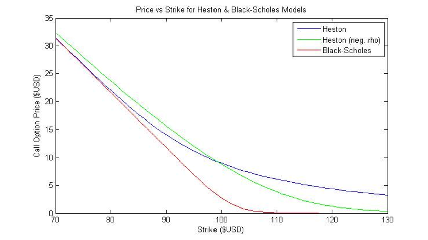
The Black-Scholes model tends to have a steeper slope as strike increases for a call option. Under a stochastic model, the outcomes can be more varied since a small change in one variable can cause a chain reaction. For instance, price increases under the Heston model can inflate volatility, further increasing the likelihood of a bigger price change. This effectively raises the uncertainty of the price of the underlying at the time of expiry which increases the associated risk of the option as well the price. Since the final price of the underlying is less certain (within the model that is), different strikes will have more similar payouts, causing a shallower slope in the graph.
Also, the premium on a call option that is very out-of-the-money remains significantly higher in the Heston model. One interpretation of this is that the stochastic nature of the Heston model makes large swings in the price of the underlying more feasible as the volatility has the potential to increase. This was also true even when a negative correlation between price and volatility was used. Intuitively, this means that if price increases, volatility is more likely to decrease. That is why the price for very out-of-the-money call options is cheaper when a negative correlation is used, however it is still significantly higher than the prices produced by the Black-Scholes model. Another relationship we analyzed was price as initial volatility changed.
Also, the premium on a call option that is very out-of-the-money remains significantly higher in the Heston model. One interpretation of this is that the stochastic nature of the Heston model makes large swings in the price of the underlying more feasible as the volatility has the potential to increase. This was also true even when a negative correlation between price and volatility was used. Intuitively, this means that if price increases, volatility is more likely to decrease. That is why the price for very out-of-the-money call options is cheaper when a negative correlation is used, however it is still significantly higher than the prices produced by the Black-Scholes model. Another relationship we analyzed was price as initial volatility changed.
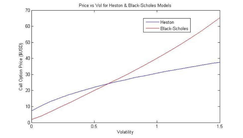
As seen, both models increase in price as volatility increases. This makes sense as the initial volatility will increase the uncertainty and risk associated with the option, thereby increasing the expected payout and price. However, the Black-Scholes model is convex while the Heston model is concave with respect to initial volatility changes. In the Black-Scholes model, the initial volatility serves as the volatility for the entire lifetime of the option. This means a high initial volatility will lead to a wide range of possible underlying prices at the time of expiry, especially for a yearly option. However, since the Heston model does not have a static volatility, changes in the initial volatility don’t have quite as big of an impact on the price. With more formalized training in stochastic calculus, the partial derivatives of the Heston model with respect to strike or volatility could be compared to those for the Black-Scholes model; however, that is outside the scope of this project. We merely attempt to note the qualitative differences via graphical analysis.
