Black Scholes
Used as the industry wide standard, the Black-Scholes model has been paramount for both traders and investors finding the theoretical “correct” price for non-dividend paying European options. The inputs for the Black-Scholes model are the underlying stock’s price, the option’s strike price, the time to the option’s expiry, the volatility of the stock, and the time value of money or in other words the risk free interest rate. The Black-Scholes model originates with the stochastic differential equation for Geometric Brownian Motion:

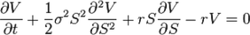
Which leads to the partial differential equation for the Black-Scholes model:
The power of the Black-Scholes model lies in the fact that there exists a closed form solution that solves the equation shown above. Traders and investors can plug the current market price of the option, strike price, time to maturity, risk free rate and underlying stock price in order to back out the implied volatility of the option. Instead of having the input volatility determine the option price, the option price implies the volatility. The implied volatility of the option is a predictor of where the market believes the volatility of the underlying stock price will be in the future. This is important because it gives traders a sense of the market sentiment for the future. In order to calculate the price of the option under the Black-Scholes model, we used the following closed form solution:

We used this solution in a slightly different form to calculate the option prices in our Monte Carlo simulations:
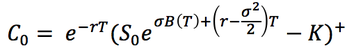
where B(T) is the Brownian motion or Wiener process, C0 and C(S,t) are the price of the call option, T is the time until maturity, σ is the volatility of the underlying stock price, r is the risk free rate, S is the price of the underlying stock, and K is the strike price. In order to test our data, we implemented this function through the following lines of MATLAB code:
final_vals=S0*exp((r-0.5*V0^2)*T + V0*sqrt(T)*randn(M,1));
option_values=max(final_vals-strike,0);
present_vals=exp(-r*T)*option_values; % Discount to present value
option_value=mean(present_vals);
option_values=max(final_vals-strike,0);
present_vals=exp(-r*T)*option_values; % Discount to present value
option_value=mean(present_vals);
where M is the
number of Monte Carlo trials and the randn
function creates a M by 1 matrix of
random variables based off of a normal distribution and V0 represents the volatility of the underlying stock price, σ. By increasing the number of Monte
Carlo trials, the error is minimized and thus our final option value is closer
to the value given by online Black-Scholes calculators. We found that choosing M = 50,000 was sufficiently high enough
to give us an accurate option value.
Heston Model
One of the major flaws in the
Black-Scholes model is the assumption that volatility will remain constant for
the life of the option. While volatility may not change drastically over small
time periods, it is very feasible that it will change over the course of a year.
The Heston model accounts for this by modeling the volatility as another
Wiener Process that has some correlation (⍴) to the price. If
the price moves, the volatility moves as well. Intuitively this makes sense: if
a large price swing occurs in a stock, the markets will be less sure of what
the true price is and the price will tend to fluctuate more. Beyond its
treatment of volatility, the Heston Model makes the same assumption as
Black-Scholes that the price changes are based on Geometric Brownian Motion.
Due to the stochastic volatility term however, the price does not reflect pure
Geometric Brownian Motion. The model also assumes that changes in the
volatility can be modelled with a normal distribution, however it incorporates
a few more variables to represent the mean-reversion tendencies of volatility.
Below are the formulas for the price and volatility under the Heston Model.
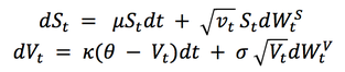
where kappa represents the mean-reversion rate, theta represents the long run volatility and σ represents the volatility of the volatility. The lower-case vt is the volatility of the price in this case. Another new parameter is the correlation factor ⍴. In order to create a Wiener Process for the volatility that is correlated to the price, we used Cholesky Decomposition, shown below.
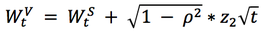
Here, Wst is the Wiener Process for the price which is just a normal distribution and z2 is another normal distribution. It is important to note that z2 has to be scaled for time to match the Wiener processes. Once we have all of these pieces, we can calculate the price of an option.
