Monte Carlo Methods
Named
after the city in Monaco famous for its casinos, the Monte Carlo method is a
popular technique used in financial mathematics to price a derivative. The
method was developed in 1946 by Stanislaw Ulam, a physicist at the Los Alamos Laboratory, and was
used to calculate radiation shielding and the distance that neutrons were
likely to travel through various materials. In finance, it is used to price
derivatives by modelling the underlying asset with some pricing process and
then simulating a “random walk”, or sample path, of the asset to obtain a
payoff for the derivative. This simulation process is then repeated many times
to represent the natural probability distribution of the payoff function. Every
payoff is converted to a fair price for the derivative. A “true value” for the
derivative is then calculated by averaging the prices from all simulations. The
Monte Carlo Method is particularly useful for pricing exotic options that are
path dependent such as American, Asian, Binary, Touch, etc.
MATLAB Optimization
As discussed, Monte Carlo simulations work by creating random price paths based on some probability distribution that will determine whether the underlying asset will increase or decrease in value and by how much. In the Black-Scholes model, a Gaussian (normal) distribution is used. However, the Black-Scholes model is used to price only European options, which can only be exercised at the time of expiry. Moreover, the payout of a European option depends only on the underlying asset’s price at the time of expiry. There are many more types of options, many of which are considered “exotic”, for which a closed-form solution such as Black-Scholes does not exist because their payout is dependent on the path of the price, not just its price at expiry.
For instance, one exotic option we looked at was the Asian option. Asian options can only be exercised at expiry but the payout is determined from the average price of the underlying asset over a given time period, making them path-dependent. While there are some closed-form approximation methods, a closed-form solution does not exist, making Monte Carlo simulations particularly useful. However, since the price at every step (namely the closing of each day) must be known, each sample path requires the generation of many random values, creating a computationally expensive problem. Optimizing this problem means that more sample paths can be used without having to wait for a computer to chug through all of the computations.
MATLAB is naturally preferred for problems like these as it is optimized for vector calculations through its use of a computer’s built-in cache system among other enhancements. However, MATLAB is an interpreted language, meaning each line of code is read and parsed in real time. Code that includes lines that are read multiple times (such is the case within loops) tends to run much slower than code that takes advantage of MATLAB’s vectorized functions. We ran into this problem with our Monte Carlo simulation for options under a Heston pricing model, which requires creating sample paths for the underlying price as well as its variance. Also, calculating the price at each step requires first calculating the price at the previous step:

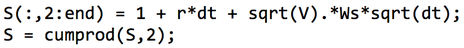
This function cannot be applied to a vector cumulatively in MATLAB without using a loop. However, we can factor out the price term to find the coefficients:

This allows us to find all of the coefficients using vector
operations and then use MATLAB’s built in cumulative product function. It is
important to note that since the variance also follows a random walk, it too is
a vector. We still need to multiply the square-root of that vector to the price
path, element wise. Instead of using a loop for this however, we can use MATLAB’s
element-wise multiplication operation ( “.*” as opposed to “*” ). After these
changes, this section of code becomes:
Besides this change, we also altered how we created and used the normally distributed random values for the price paths as well as the correlated variance paths. Initially we created a set of Mv variance paths and a set of Ms price paths and then used every variance path with every price path for a total of M = Mv*Ms simulations. However, this required using nested loops, which is particularly slow in MATLAB. We opted to give up the space efficiency of this method, which was marginal to begin with, for speed by creating M variance and price paths. Since we could now use built in element-wise operations, our code ran much faster. Below is a table showing the difference in run times between our optimized and non-optimized code.
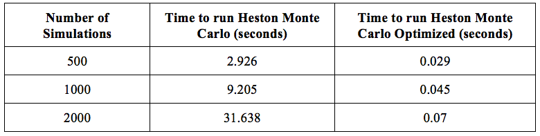
Clearly, the optimized code runs significantly faster, especially when we run a large number of simulations. With 2000 simulations, the optimized code runs about 450 times faster than the non-optimized code. With the ability to run more simulations faster, the accuracy of a Monte Carlo simulation increases greatly.
